A new E-score for KrakenUniq

using the double-exponential function

May 10, 2022 7 min read

Introduction

The task of taxonomic profiling consists of answering the question “Who is there ?" in a metagenomic sample. However, in practice, it turns out to be quite a challenging assignment to tackle, and many solutions have been proposed to address it (for a comparative benchmark, see Meyer et al. 2022).

One of the central aspect of taxonomic profiling is to distinguishing true positive (taxon actually present in a sample) from false positive (taxon not actually present in sample) taxonomic assignments.

Today, I want to focus on one particular taxonomic profiler: KrakenUniq (Breitwieser et al. 2018).

Based on the popular k-mer based taxonomic classifier Kraken (Wood et al. 2014), KrakenUniq adds a unique (😉) feature on top of Kraken, the reporting of unique k-mer counts.

Let me explain:

The original Kraken program is based on direct k-mer matching. First Kraken builds a database of all present k-mer in each reference genomes, and then compares it to the k-mers found in the query sequences/sequencing reads (fig 1) . If there is a match, it uses a taxonomic tree and the LCA algorithm to assign each query sequence to a given taxon.

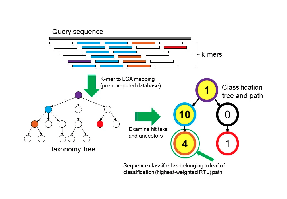
Figure 1: The Kraken sequence classification algorithm. original here

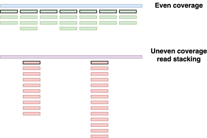
While this is already a good performing taxonomic profiling method, it suffers from one major drawback: it can not account for duplicated sequences. For example, when reporting the number of reads belonging to each taxon in a sample, Kraken is not able to distinguish an evenly covered genome (likely a true positive, blue genome fig 2) from a genome suffering from read stacking (likely a false positive, purple genome, fig 2). This uneven coverage, often a false positive assignment, can be the consequence of different reasons, but one of the most common is due to reads matching ultra-conserved regions between taxons from the same clade, the so-called read stacking.

Figure 2: Two taxons having the same amount of assigned reads, two different scenarios. The blue genome has an evenly distributed coverage, while the purple genome suffers from read stacking. Unique kmers are highlighted with a black perimeter

To circumvent this problem, KrakenUniq leverages the HLL algorithm to count the unique/distinct k-mers. In practice, in the example of fig 2, Kraken would have reported a k-mer count of 24 for both the blue and purple genome, while KrakenUniq would have reported a k-mer count of 7 for the blue genome, and k-mer count of 2 for the purple genome.

On top of that, KrakenUniq keeps track of how many of unique k-mers have been found, out all possible unique k-mers for each taxon, and normalizes it by the taxon genome size, which gives an estimation of the “coverage”.

So, to summarize, with KrakenUniq, for each taxon, we now have three different metrics instead of “just one” for Kraken :

read count per taxon (which we already had with kraken), we’ll refer to it later as $R$
number of unique k-mers (new with KrakenUniq), we’ll refer to it later as $K$
“coverage” of the k-mers of the clade in the database, we’ll refer to it later as $C$

Note that I’ve always mentioned the “coverage” between quotes, this is because KrakenUniq defines it as $C = \frac{K}{genome\ size}$.
Because by definition, the maximum number of k-mers (of length $k$) for a sequence of length $L$ can not exceed $L - k + 1$. This means that in the ideal situation, for example the blue genome of fig 2, the “coverage” will be at best, close to 1, but never greater than 1.

To try to make sense of these three metrics, Guellil et al. 2022 came up with a score $E$ combining them, to discriminate true positive from false positive taxonomic assignments.

$$E = \frac{K}{R} \times C$$

Here, using different simulated taxon assignment situations, I propose a tweak to this score, to try to improve its ability to differentiate true positive from false positive taxonomic assignments.

The simulations

First, let’s define a few parameters for our simulation, and import necessary libraries

import numpy as np
import matplotlib.pyplot as plt
import seaborn as sns
import pandas as pd

read_length = 45
kmer_length = 35
genome_size = 1000000

We’ll look at four different possible scenarios
For each scenario, we’ll simulate 100 different situations

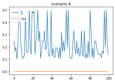
scenario A: high duplication, low coverage (false positive)

A lot of reads are duplicated, probably coming from conversed regions, or sequencing artifacts
low coverage
There are more reads than unique k-mers

a_reads = np.random.randint(10, 300, 100) # randomly choose the number of reads, between 10 and 300
comp_kmer_a = lambda x: int(x / np.random.randint(2,10, 1))  # randomly choose between 2 and 10 times less k-mers
comp_kmer_a_vec = np.vectorize(comp_kmer_a)
a_kmers = comp_kmer_a_vec(a_reads)
plt.plot(a_kmers/a_reads, label=r"$\frac{k}{R}$")
plt.plot(a_kmers/genome_size, label="cov")
plt.title("scenario A")
plt.legend(loc="upper left");

png

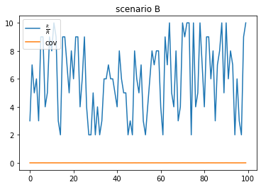
scenario B: low duplication, low coverage (true positive)

Very few reads are duplicated
low coverage
more unique k-mers than reads (up to $ku = read_length - kmer_length + 1$ more unique k-mers than reads)

b_reads = np.random.randint(10, 300, 100) # randomly choose the number of reads, between 10 and 300
comp_kmer_b = lambda x: min(genome_size - kmer_length + 1, int(x * np.random.randint(2,(read_length - kmer_length + 1), 1))) # randomly choose up to ku more k-mers than reads
comp_kmer_b_vec = np.vectorize(comp_kmer_b)
b_kmers = comp_kmer_b_vec(b_reads)

plt.plot(b_kmers/b_reads, label=r"$\frac{k}{R}$")
plt.plot(b_kmers/genome_size, label="cov")
plt.title("scenario B")
plt.legend(loc="upper left");

png

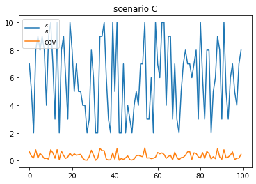
scenario C: low duplication, higher coverage (true positive)

same as scenario B, but with a higher coverage

c_reads = np.random.randint(10000, 100000, 100) # # randomly choose the number of reads, between 10000 and 100000
comp_kmer_c = lambda x: min(genome_size - kmer_length + 1, int(x * np.random.randint(2,(read_length - kmer_length + 1), 1)))
comp_kmer_c_vec = np.vectorize(comp_kmer_c)
c_kmers = comp_kmer_c_vec(c_reads)
plt.plot(c_kmers/c_reads, label=r"$\frac{k}{R}$")
plt.plot(c_kmers/genome_size, label="cov")
plt.title("scenario C")
plt.legend(loc="upper left");

png

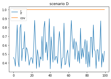
scenario D: low duplication, high coverage

more reads than unique kmers (because of the coverage definiton of KrakenUniq)
high coverage

d_reads = np.random.randint(genome_size*1.1, genome_size*3, 100) # getting between 1.1*genome_size and 3*genome size reads
comp_kmer_d = lambda x: min(genome_size - kmer_length + 1, int(x * np.random.randint(2,(read_length - kmer_length + 1), 1)))
comp_kmer_d_vec = np.vectorize(comp_kmer_d)
d_kmers = comp_kmer_d_vec(d_reads)
plt.plot(d_kmers/d_reads, label=r"$\frac{k}{R}$")
plt.plot(d_kmers/genome_size, label="cov")
plt.title("scenario D")
plt.legend(loc="upper left");

png

Comparing E-scores

Guellil et al. E-score

Now that we have our four different scenarios, let’s look at how Guellil et al. E-score performs at discriminating between true positive (scenario A) and false positive (scenario B, C, and D) taxonomic assignments.

def e_score_guellil(nb_kmer, nb_read, genome_size):
    cov = nb_kmer/genome_size
    
    return((nb_kmer/nb_read) * cov )
e_score_guellil_vec = np.vectorize(e_score_guellil)

e_score_guellil_a = e_score_guellil_vec(a_kmers, a_reads, genome_size)
e_score_guellil_b = e_score_guellil_vec(b_kmers, b_reads, genome_size)
e_score_guellil_c = e_score_guellil_vec(c_kmers, c_reads, genome_size)
e_score_guellil_d = e_score_guellil_vec(d_kmers, d_reads, genome_size)

plt.plot(e_score_guellil_a, label = "scenario A")
plt.plot(e_score_guellil_b, label = "scenario B")
plt.plot(e_score_guellil_c, label = "scenario C")
plt.plot(e_score_guellil_d, label = "scenario D")
plt.legend(loc="upper left")
plt.title("Guellil et al. E score")
plt.ylim(0,0.001);

png

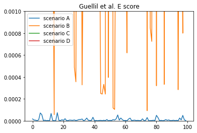
As we can see, it can be quite tricky in some situations to differentiate a true from a false positive assignment. This is particularly problematic between scenario A and scenario B.

Modified dexp E-score

Here I propose a slightly different score to mitigate some of issue. Instead of defining

$$E = \frac{K}{R}\times C$$

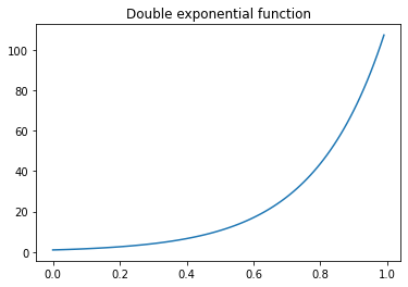
I propose to use

$$E = \frac{K}{R} \times dexp(C)$$

with $dexp$ being the double exponential function.

This way, more emphasis is given to the “coverage”, which particularly helps in low “coverage” scenarios, since the double exponential function grows “really fast” between 0 and 1.

#https://en.wikipedia.org/wiki/Double_exponential_function
def double_exp(x, a=1.3, b=18):
    return(a**(b*x))
double_exp_vec = np.vectorize(double_exp)

x = np.arange(0,1,0.01)
y = double_exp_vec(x)
plt.plot(x, y)
plt.title("Double exponential function");

png

def e_score_dexp(nb_kmer, nb_read, genome_size):
    cov = nb_kmer/genome_size
    
    return((nb_kmer/nb_read) * double_exp(cov))
e_score_dexp_vec = np.vectorize(e_score_dexp)

Now let’s look at how this modified E-score performs

e_score_dexp_a = e_score_dexp_vec(a_kmers, a_reads, genome_size)
e_score_dexp_b = e_score_dexp_vec(b_kmers, b_reads, genome_size)
e_score_dexp_c = e_score_dexp_vec(c_kmers, c_reads, genome_size)
e_score_dexp_d = e_score_dexp_vec(d_kmers, d_reads, genome_size)

plt.plot(e_score_dexp_a, label = "case_a")
plt.plot(e_score_dexp_b, label = "case_b")
plt.plot(e_score_dexp_c, label = "case_c")
plt.plot(e_score_dexp_d, label = "case_b")
plt.legend(loc="upper left")
plt.title("Double-exp E-score")

plt.ylim(0,4);

png

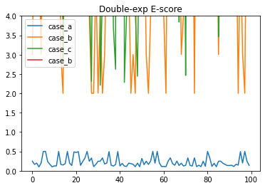
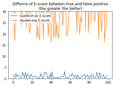
We can see that there is a much clearer distinction between true and false positive assignments. We can also look at the mean difference of all scenarios between true and false positives, for the original, and the new double exp E-score

diff_e_score_guellil = np.mean([e_score_guellil_b - e_score_guellil_a, e_score_guellil_c - e_score_guellil_a, e_score_guellil_d - e_score_guellil_a], axis=0)
diff_e_score_dexp = np.mean([e_score_dexp_b - e_score_dexp_a, e_score_dexp_c - e_score_dexp_a, e_score_dexp_d - e_score_dexp_a], axis=0)

plt.plot(diff_e_score_guellil, label="Guellil et al. E-score")
plt.plot(diff_e_score_dexp, label="double-exp E-score")
plt.title("Difference of E-score between true and false positive\n(the greater the better)")
plt.legend(loc="upper left")
plt.ylim(0,30);

png

df = pd.DataFrame(list(zip(diff_e_score_guellil, diff_e_score_dexp)), columns=['Guellil et al.', 'dexp'])

sns.boxplot(data=df)
plt.title("Difference of E-score between true and false positive\n(the greater the better)");

png

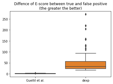
df.mean(axis=0)

Guellil et al.     1.012888
dexp              50.104112
dtype: float64

We can see that on average between all scenarios, for Guellil et al. E-score, there is only a difference of 1 point, while for the modified double-exponential E-score, there is an average difference of 50 points.

Conclusion

In my simulations, using a the modified double-exponential E-score could allow for a better distinction between true and false positive taxonomic assignations by KrakenUniq.

The notebook used for this blog post is available here